11 Fehlermasse

11.1 Bias

\(\text{Bias}_{\text{additiv}} = \bar{\text{Vorhersage}} - \bar{\text{Beobachtung}}\)
\(\text{Bias}_{\text{multiplikativ}} = \frac{\bar{\text{Vorhersage}}}{\bar{\text{Beobachtung}}}\)

Code

import matplotlib.pyplot as plt

# Funktion zum Zeichnen eines "Zielscheiben"-Diagramms mit Punkten
def draw_target(ax, points, title, label_y=None):
    # Zeichnen der Zielscheibe (zwei konzentrische Kreise)
    target = plt.Circle((0, 0), 1, color='black', fill=False, lw=1.5)
    inner_circle = plt.Circle((0, 0), 0.3, color='black', fill=False, lw=1.5)
    ax.add_artist(target)
    ax.add_artist(inner_circle)

    # Punkte hinzufügen
    for (x, y) in points:
        ax.plot(x, y, 'ko', markersize=8)

    # Formatierung
    ax.set_xlim(-1.5, 1.5)
    ax.set_ylim(-1.5, 1.5)
    ax.set_aspect('equal')
    ax.axis('off')
    ax.set_title(title, fontsize=12)

    if label_y:
        ax.text(-2.5, 0, label_y, va='center', ha='center', rotation=90, fontsize=12, fontweight='bold')

# Punkte für jede der vier Kategorien
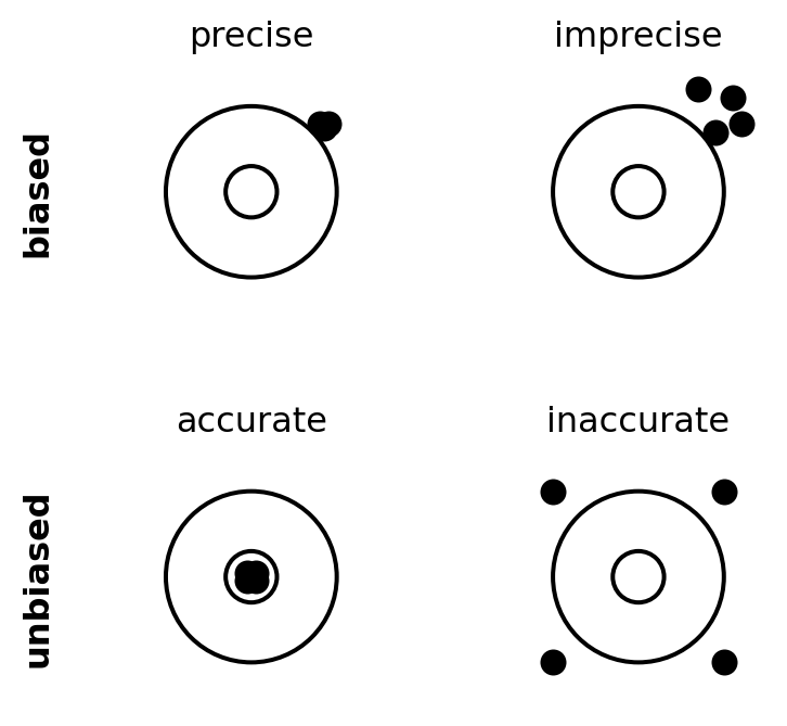
points_precise_biased = [(0.8, 0.8), (0.85, 0.75), (0.9, 0.8)]
points_imprecise_biased = [(1.1, 1.1), (0.9, 0.7), (1.2, 0.8), (0.7, 1.2)]
points_precise_unbiased = [(0.05, 0.05), (-0.05, 0.05), (0.05, -0.05), (-0.05, -0.05)]
points_imprecise_unbiased = [(-1, 1), (1, -1), (-1, -1), (1, 1)]

# Erstellen des 2x2 Plots
fig, axs = plt.subplots(2, 2, figsize=(4, 4))

# Obere Reihe (biased)
draw_target(axs[0, 0], points_precise_biased, "precise", label_y="biased")
draw_target(axs[0, 1], points_imprecise_biased, "imprecise")

# Untere Reihe (unbiased)
draw_target(axs[1, 0], points_precise_unbiased, "accurate", label_y="unbiased")
draw_target(axs[1, 1], points_imprecise_unbiased, "inaccurate")

# Layout anpassen
plt.subplots_adjust(wspace=0.5, hspace=0.5)

plt.show()

11.2 Mittlerer absoluter Fehler (MAE)

\[ \begin{align*} \operatorname{MAE} &= \frac{1}{N} \sum_{i=1}^{N} |\hat{y}_i - y_i| \\ \operatorname{MAE} &= \frac{1}{N} \sum_{i=1}^{N} |\text{Vorhersage}_i - \text{Beobachtung}_i| \end{align*} \]

11.3 Mittlerer quadratischer Fehler (MSE)

\[ \begin{align*} \operatorname{MSE} &= \frac{1}{N} \sum_{i=1}^{N} (\hat{y}_i - y_i)^2 \\ \operatorname{MSE} &= \frac{1}{N} \sum_{i=1}^{N} (\text{Vorhersage}_i - \text{Beobachtung}_i)^2 \end{align*} \]

oft wird noch die Wurzel gezogen, um wieder die gleiche Einheit wie die Beobachtung zu erhalten:

\[ \operatorname{RMSE} = \sqrt{\frac{1}{N} \sum_{i=1}^{N} (\hat{y}_i - y_i)^2} \]

Hier bekommen grosse Abweichungen mehr gewicht, als beim MAE.