7 Verteilungen

Ereignisraum, Wahrscheinlichkeit, Zufallsvariable

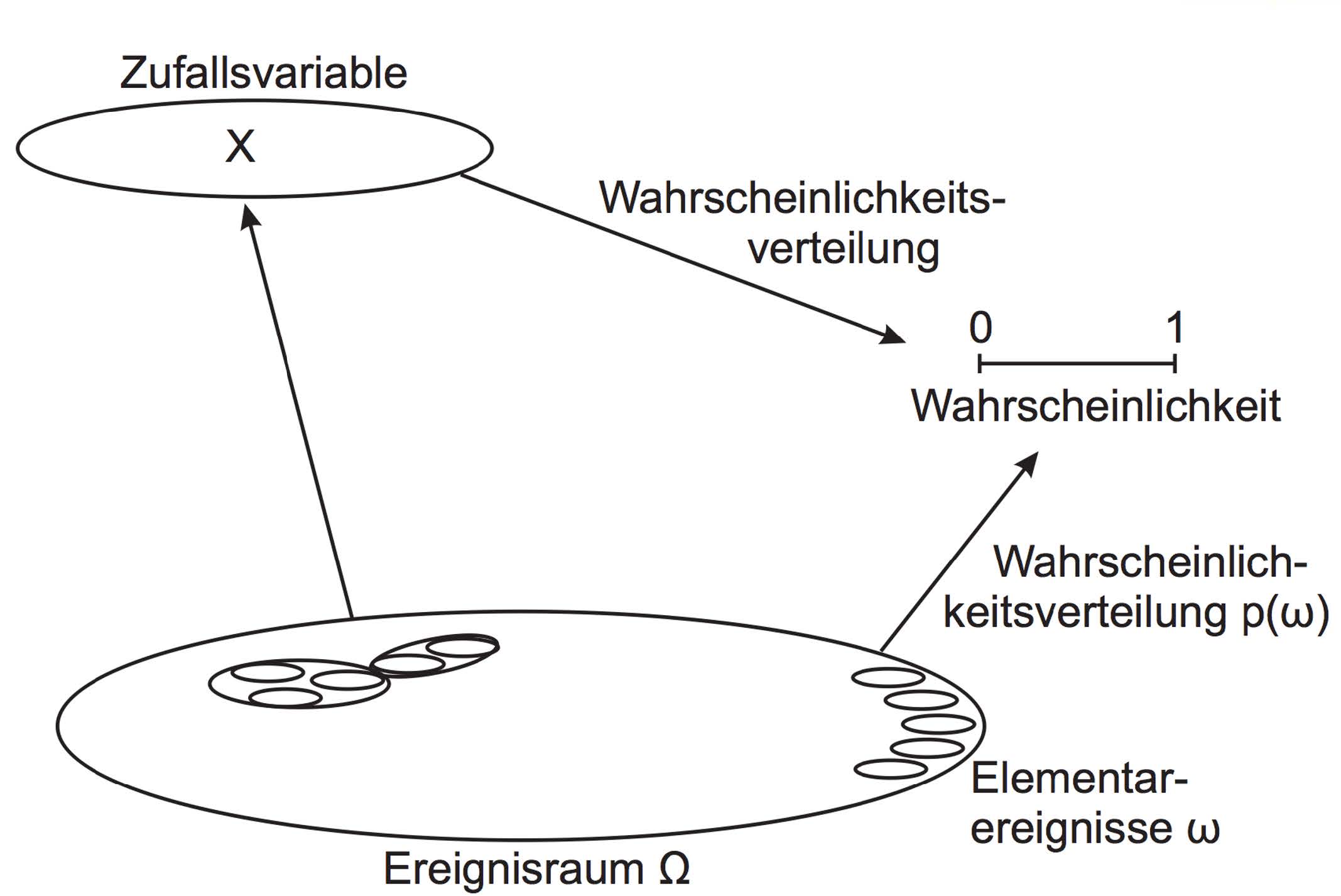
Zufallsvariable \(X\): Variable die den Ergebnissen eines Zufallsexperiments Werte (Realisierungen) zuordnet
Wahrscheinlichkeit \(P\): theoretische Häufigkeit, mit der ein Ereignis in einer grossen Anzahl gleicher, wiederholter, voneinander unabhängiger Zufallsexperimente auftritt (z.B. 0.5 für Zahl beim Münzwurf)
Ereignisraum \(\Omega\): Alle theoretisch möglichen Ereignisse, denen sich Wahrscheinlichkeiten zuordnen lassen
Elementarereignisse \(\omega\): Ergebnis eines Zufallsexperiments
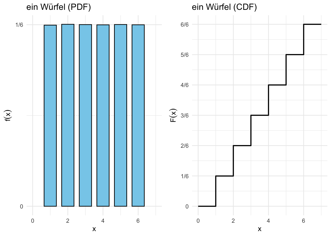
Wahrscheinlichkeitsfunktion \(f(x)\): Funktion, die jedem Ereignis \(\omega\) eine Wahrscheinlichkeit \(P(\omega)\) zuordnet
Verteilungsfunktion \(F(x)\): Funktion, die die Wahrscheinlichkeit angibt, dass die Zufallsvariable \(X\) einen Wert kleiner oder gleich \(x\) annimmt
Wahrscheinlichkeitsverteilung \(p(\omega)\): Wahrscheinlichkeit, dass das Ereignis \(\omega\) eintritt

7.1 Theoretische Verteilungen diskreter Zufallsvariablen

7.1.1 Diskrete Gleichverteilung

Code

library(ggplot2)
library(dplyr)
library(gridExtra)

# Funktion zum Berechnen der Wahrscheinlichkeits- und Verteilungsfunktionen
simulate_dice <- function(n_dice) {
  rolls <- replicate(1000000, sum(sample(1:6, n_dice, replace = TRUE)))  # Simulation von n_dice Würfeln
  df <- as.data.frame(table(rolls) / length(rolls)) %>%
    rename(x = rolls, probability = Freq) %>%
    mutate(x = as.numeric(as.character(x))) %>%
    arrange(x) %>%
    mutate(cumulative_probability = cumsum(probability))

  # Zusätzliche Punkte für 0 und 1
  df <- rbind(data.frame(x = 0, probability = 0, cumulative_probability = 0),
              df,
              data.frame(x = max(df$x) + 1, probability = 0, cumulative_probability = 1))
  return(df)
}

# Daten für 1 Würfel
df_1dice <- simulate_dice(1)

# Plot für die Wahrscheinlichkeitsfunktion (PDF) von 1 Würfel
plot_pdf_1 <- ggplot(df_1dice, aes(x = x, y = probability)) +
  geom_bar(stat = "identity", fill = "skyblue", color = "black", width = 0.7) +
  labs(title = "ein Würfel (PDF)", x = "x", y = expression(f(x))) +
  theme_minimal() +
  ylim(0, max(df_1dice$probability, na.rm = TRUE) * 1.1) +
  xlim(0, 7) +
  scale_y_continuous(breaks = seq(0, 1/6, by = 1/6),
                    labels = c("0", "1/6"))

# Plot für die kumulative Verteilungsfunktion (CDF) von 1 Würfel
plot_cdf_1 <- ggplot(df_1dice, aes(x = x, y = cumulative_probability)) +
  geom_step(linewidth = 0.8, color = "black") +
  labs(title = "ein Würfel (CDF)", x = "x", y = expression(F(x))) +
  theme_minimal() +
  ylim(0, 1) +
  xlim(0, 7) +
  scale_y_continuous(breaks = seq(0, 1, by = 1/6),
                    labels = c("0", "1/6", "2/6", "3/6", "4/6", "5/6", "6/6"))

# Anordnung der beiden Plots in einem 2x1-Layout
grid.arrange(plot_pdf_1, plot_cdf_1, ncol = 2)

Abbildung 7.1: Diskrete Wahrscheinlichkeits- und Verteilungsfunktionen für einen Würfel (Berechnet mit 1’000’000 Simulationen)

Code

library(ggplot2)
library(dplyr)
library(gridExtra)

# Funktion zum Berechnen der Wahrscheinlichkeits- und Verteilungsfunktionen
simulate_dice <- function(n_dice) {
  rolls <- replicate(10000, sum(sample(1:6, n_dice, replace = TRUE)))  # Simulation von n_dice Würfeln
  df <- as.data.frame(table(rolls) / length(rolls)) %>%
    rename(x = rolls, probability = Freq) %>%
    mutate(x = as.numeric(as.character(x))) %>%
    arrange(x) %>%
    mutate(cumulative_probability = cumsum(probability))
  return(df)
}

# Daten für 2, 3 und 4 Würfel
df_2dice <- simulate_dice(2)
df_3dice <- simulate_dice(3)
df_4dice <- simulate_dice(4)

# Plots für die PDF und CDF von 2 Würfeln
plot_pdf_2 <- ggplot(df_2dice, aes(x = x, y = probability)) +
  geom_bar(stat = "identity", fill = "skyblue", color = "black", width = 0.7) +
  labs(title = "zwei Würfel (PDF)", x = "x", y = expression(f(x))) +
  theme_minimal() +
  ylim(0, max(df_2dice$probability, na.rm = TRUE) * 1.1)

plot_cdf_2 <- ggplot(df_2dice, aes(x = x, y = cumulative_probability)) +
  geom_step(linewidth = 0.8, color = "black") +
  labs(title = "zwei Würfel (CDF)", x = "x", y = expression(F(x))) +
  theme_minimal() +
  ylim(0, 1)

# Plots für die PDF und CDF von 3 Würfeln
plot_pdf_3 <- ggplot(df_3dice, aes(x = x, y = probability)) +
  geom_bar(stat = "identity", fill = "skyblue", color = "black", width = 0.7) +
  labs(title = "drei Würfel (PDF)", x = "x", y = expression(f(x))) +
  theme_minimal() +
  ylim(0, max(df_3dice$probability, na.rm = TRUE) * 1.1)

plot_cdf_3 <- ggplot(df_3dice, aes(x = x, y = cumulative_probability)) +
  geom_step(linewidth = 0.8, color = "black") +
  labs(title = "drei Würfel (CDF)", x = "x", y = expression(F(x))) +
  theme_minimal() +
  ylim(0, 1)

# Plots für die PDF und CDF von 4 Würfeln
plot_pdf_4 <- ggplot(df_4dice, aes(x = x, y = probability)) +
  geom_bar(stat = "identity", fill = "skyblue", color = "black", width = 0.7) +
  labs(title = "vier Würfel (PDF)", x = "x", y = expression(f(x))) +
  theme_minimal() +
  ylim(0, max(df_4dice$probability, na.rm = TRUE) * 1.1)

plot_cdf_4 <- ggplot(df_4dice, aes(x = x, y = cumulative_probability)) +
  geom_step(linewidth = 0.8, color = "black") +
  labs(title = "vier Würfel (CDF)", x = "x", y = expression(F(x))) +
  theme_minimal() +
  ylim(0, 1)

# Anordnung der Plots in einem 3x2-Layout
grid.arrange(plot_pdf_2, plot_pdf_3, plot_pdf_4, plot_cdf_2, plot_cdf_3, plot_cdf_4, ncol = 3, nrow = 2)

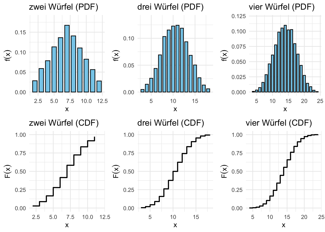
Abbildung 7.2: Diskrete Wahrscheinlichkeits- und Verteilungsfunktionen für 2, 3 und 4 Würfel (Berechnet mit 100’000 Simulationen)

Mit mehr Würfeln kommt das immer näher an eine Normalverteilung

Code

# Lade benötigte Pakete
library(ggplot2)
library(dplyr)
library(gridExtra)

# Parameter definieren
n_dice <- 15       # Anzahl Würfel
n_simulations <- 100000  # Anzahl Simulationen

# Dynamische xlim basierend auf minimaler/maximaler Würfelsumme
x_min <- n_dice * 1      # Minimale Summe (alle Würfel = 1)
x_max <- n_dice * 6      # Maximale Summe (alle Würfel = 6)

# Funktion zur Simulation der Würfelsummen und Berechnung der Wahrscheinlichkeiten
simulate_dice <- function(n_dice, n_simulations) {
  
  # Simulation: Summe von n_dice Würfeln pro Durchlauf
  rolls <- replicate(n_simulations, sum(sample(1:6, n_dice, replace = TRUE)))
  
  # Häufigkeitstabelle mit Wahrscheinlichkeiten und kumulativen Wahrscheinlichkeiten
  df <- as.data.frame(table(rolls)) %>%
    rename(x = rolls, probability = Freq) %>%
    mutate(
      x = as.numeric(as.character(x)),         # x als numerisch
      probability = probability / sum(probability),   # Wahrscheinlichkeiten normieren
      cumulative_probability = cumsum(probability)     # Kumulative Verteilungsfunktion
    ) %>%
    arrange(x)
  
  return(df)
}

# Simulation durchführen
df_results <- simulate_dice(n_dice, n_simulations)

# Wahrscheinlichkeitsfunktion (PDF) plotten
plot_pdf <- ggplot(df_results, aes(x = x, y = probability)) +
  geom_bar(stat = "identity", fill = "skyblue", color = "black", width = 0.7) +
  labs(
    title = paste(n_dice, "Würfel (PDF)"),
    x = "Summe der Würfel",
    y = expression(f(x))
  ) +
  theme_minimal() +
  # x-Achse dynamisch setzen
  xlim(c(x_min, x_max))

# Kumulative Verteilungsfunktion (CDF) plotten
plot_cdf <- ggplot(df_results, aes(x = x, y = cumulative_probability)) +
  geom_step(linewidth = 0.8, color = "black") +
  labs(
    title = paste(n_dice, "Würfel (CDF)"),
    x = "Summe der Würfel",
    y = expression(F(x))
  ) +
  theme_minimal() +
  ylim(0, 1) +
  # x-Achse dynamisch setzen
  xlim(c(x_min, x_max))

# Beide Plots nebeneinander ausgeben
grid.arrange(plot_pdf, plot_cdf, ncol = 2)

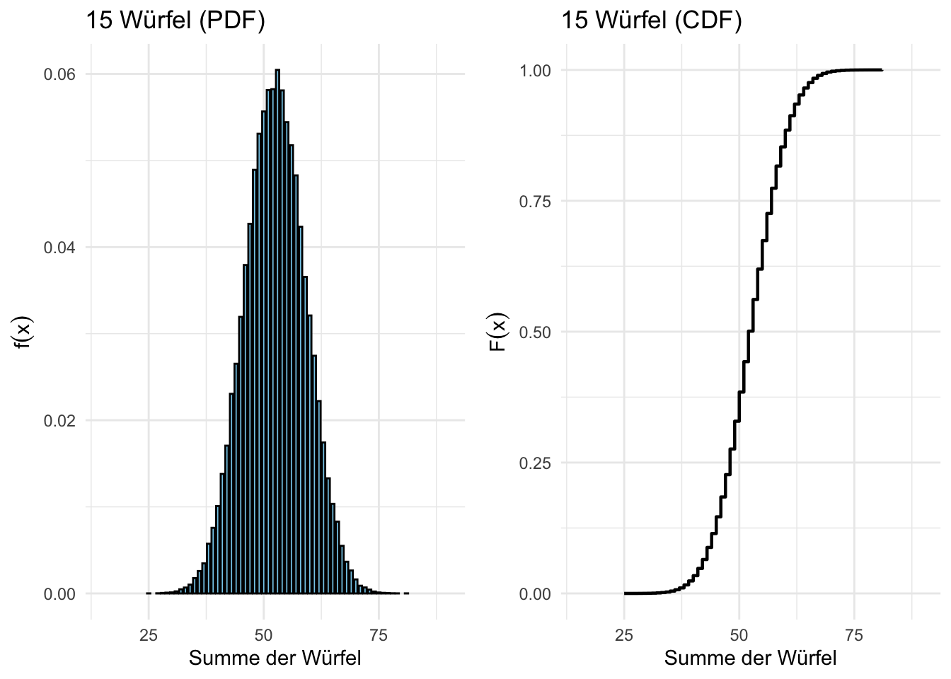
Abbildung 7.3: Diskrete Wahrscheinlichkeits- und Verteilungsfunktionen für 15 Würfel (Berechnet mit 100’000 Simulationen)

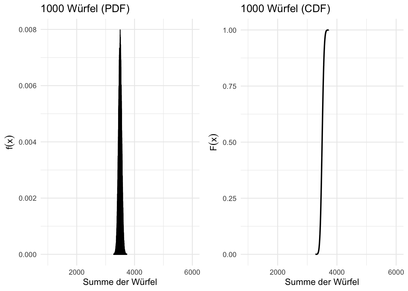
Was passiert bei extrem vielen Würfeln?

Spannend ist dass die Streuung der Summen extrem klein wird.

Code

# Lade benötigte Pakete
library(ggplot2)
library(dplyr)
library(gridExtra)

# Parameter definieren
n_dice <- 1000       # Anzahl Würfel
n_simulations <- 100000  # Anzahl Simulationen

# Dynamische xlim basierend auf minimaler/maximaler Würfelsumme
x_min <- n_dice * 1      # Minimale Summe (alle Würfel = 1)
x_max <- n_dice * 6      # Maximale Summe (alle Würfel = 6)

# Funktion zur Simulation der Würfelsummen und Berechnung der Wahrscheinlichkeiten
simulate_dice <- function(n_dice, n_simulations) {
  
  # Simulation: Summe von n_dice Würfeln pro Durchlauf
  rolls <- replicate(n_simulations, sum(sample(1:6, n_dice, replace = TRUE)))
  
  # Häufigkeitstabelle mit Wahrscheinlichkeiten und kumulativen Wahrscheinlichkeiten
  df <- as.data.frame(table(rolls)) %>%
    rename(x = rolls, probability = Freq) %>%
    mutate(
      x = as.numeric(as.character(x)),         # x als numerisch
      probability = probability / sum(probability),   # Wahrscheinlichkeiten normieren
      cumulative_probability = cumsum(probability)     # Kumulative Verteilungsfunktion
    ) %>%
    arrange(x)
  
  return(df)
}

# Simulation durchführen
df_results <- simulate_dice(n_dice, n_simulations)

# Wahrscheinlichkeitsfunktion (PDF) plotten
plot_pdf <- ggplot(df_results, aes(x = x, y = probability)) +
  geom_bar(stat = "identity", fill = "skyblue", color = "black", width = 0.7) +
  labs(
    title = paste(n_dice, "Würfel (PDF)"),
    x = "Summe der Würfel",
    y = expression(f(x))
  ) +
  theme_minimal() +
  # x-Achse dynamisch setzen
  xlim(c(x_min, x_max))

# Kumulative Verteilungsfunktion (CDF) plotten
plot_cdf <- ggplot(df_results, aes(x = x, y = cumulative_probability)) +
  geom_step(linewidth = 0.8, color = "black") +
  labs(
    title = paste(n_dice, "Würfel (CDF)"),
    x = "Summe der Würfel",
    y = expression(F(x))
  ) +
  theme_minimal() +
  ylim(0, 1) +
  # x-Achse dynamisch setzen
  xlim(c(x_min, x_max))

# Beide Plots nebeneinander ausgeben
grid.arrange(plot_pdf, plot_cdf, ncol = 2)

Abbildung 7.4: Diskrete Wahrscheinlichkeits- und Verteilungsfunktionen für 1000 Würfel (Berechnet mit 100’000 Simulationen)

7.1.2 Normalverteilung

Zentraler Grenzwertsatz

\[ \lim_{n \to \infty} \frac{1}{n} \sum_{i=1}^{n} X_i = \mu \]

Der Zentrale Grenzwertsatz besagt, dass die Summe von unabhängigen, identisch verteilten Zufallsvariablen mit wachsendem \(n\) gegen eine Normalverteilung konvergiert.

\[ f_{\mu, \sigma}(x) = \frac{1}{\sigma \sqrt{2\pi}} e^{-\frac{(x-\mu)^2}{2\sigma^2}} \]

Code

library(ggplot2)
library(gridExtra)

# Erzeugung der Normalverteilung
x <- seq(-4, 4, length.out = 1000)
y_pdf <- dnorm(x, mean = 0, sd = 1)
y_cdf <- pnorm(x, mean = 0, sd = 1)

# Datensätze erstellen
df_pdf <- data.frame(x = x, y = y_pdf)
df_cdf <- data.frame(x = x, y = y_cdf)

# PDF Plot
plot_pdf <- ggplot(df_pdf, aes(x = x, y = y)) +
  geom_ribbon(data = subset(df_pdf, x >= -3 & x <= 3),
             aes(ymin = 0, ymax = y, fill = "99.73%")) +
  geom_ribbon(data = subset(df_pdf, x >= -2 & x <= 2),
             aes(ymin = 0, ymax = y, fill = "95.45%")) +
  geom_ribbon(data = subset(df_pdf, x >= -1 & x <= 1),
             aes(ymin = 0, ymax = y, fill = "68.27%")) +
  geom_line(linewidth = 1) +
  geom_vline(xintercept = c(-3, -2, -1, 1, 2, 3), 
            linetype = "dashed", color = "gray40") +
  labs(x = "Standardabweichungen (σ)", 
       y = "f(x)",
       title = "Dichtefunktion") +
  scale_x_continuous(breaks = -3:3,
                    labels = paste0(c("-3", "-2", "-1", "0", "1", "2", "3"), "σ")) +
  scale_fill_manual(values = c(
    "68.27%" = "#2C7BB6",
    "95.45%" = "#81B9D9",
    "99.73%" = "#D1E5F0"
  )) +
  theme_minimal() +
  theme(
    panel.grid.minor = element_blank(),
    legend.position = "bottom",
    legend.title = element_blank()
  )

# CDF Plot
plot_cdf <- ggplot(df_cdf, aes(x = x, y = y)) +
  geom_line(linewidth = 1) +
  geom_vline(xintercept = c(-3, -2, -1, 1, 2, 3), 
            linetype = "dashed", color = "gray40") +
  labs(x = "Standardabweichungen (σ)", 
       y = "F(x)",
       title = "Verteilungsfunktion") +
  scale_x_continuous(breaks = -3:3,
                    labels = paste0(c("-3", "-2", "-1", "0", "1", "2", "3"), "σ")) +
  scale_y_continuous(breaks = seq(0, 1, 0.2)) +
  theme_minimal() +
  theme(
    panel.grid.minor = element_blank()
  )

# Plots nebeneinander anordnen
grid.arrange(plot_pdf, plot_cdf, ncol = 2)

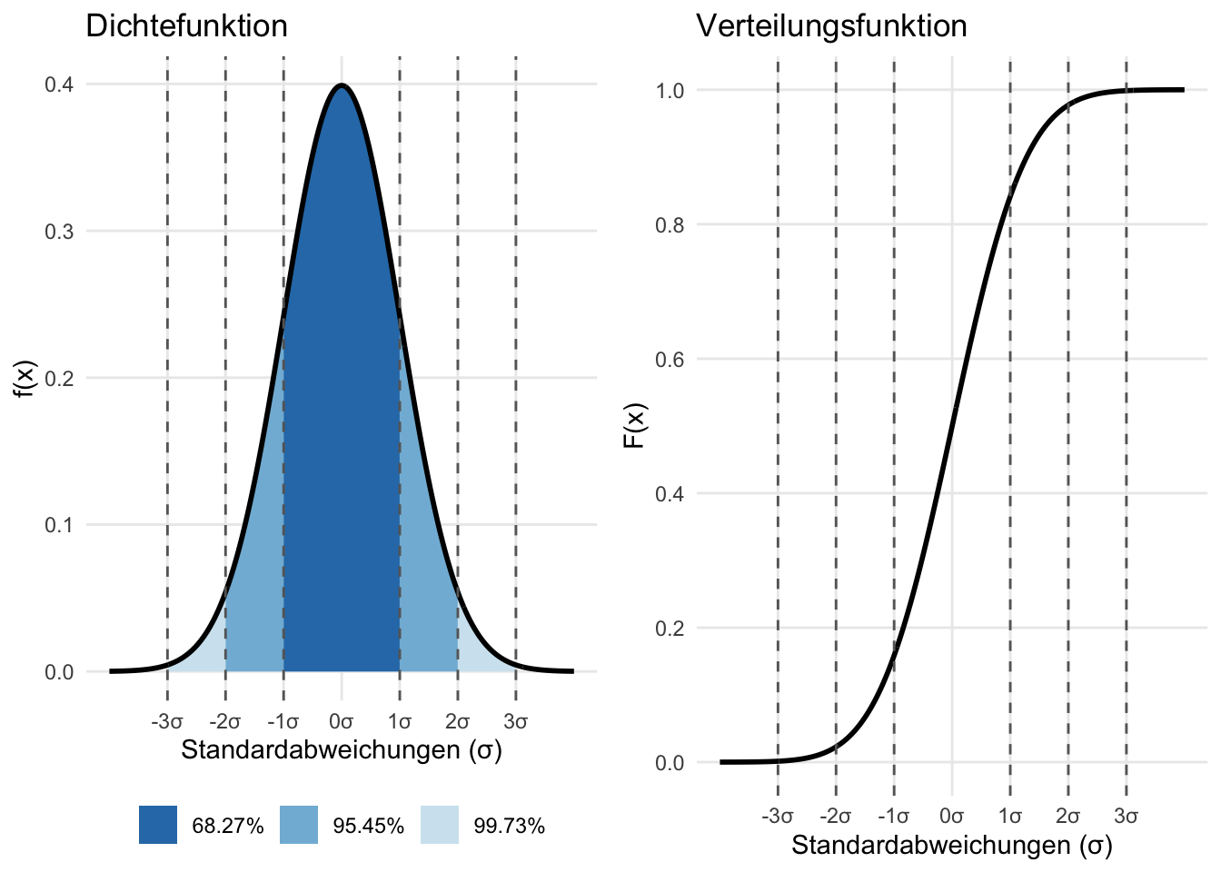
Abbildung 7.5: Links: Wahrscheinlichkeitsdichte (PDF), Rechts: Verteilungsfunktion (CDF) der Normalverteilung

Symmetrisch zur Achse \(x = \mu\)
unimodal mit Maximum bei \(x = \mu\)
Wendepunkte bei \(x = \mu \pm \sigma\)
asymptotisch gegen 0

7.1.2.1 Standardisierung

Durch eine Transformation zu \(\mu = 0\) und \(\sigma = 1\) erhält man eine standardisierte Zufallsvariable.

\[ z = \frac{X - \mu}{\sigma} \]

Wobei \(z\) die standardisierte Zufallsvariable, \(X\) die ursprüngliche Zufallsvariable und \(\mu\) und \(\sigma\) der Mittelwert und die Standardabweichung der ursprünglichen Verteilung sind.

Die Standardisierung wird verwendet, um verschiedene Elemente (d.h. Daten mit Bias oder unterschiedlichen Einheiten oder unterschiedlicher Varianz, etc.) zu vergleichen.

Beispiel

Angenommen, wir haben eine Stichprobe von 5 Studierenden und ihre Prüfungsnoten (Skala 0–100):

Tabelle 7.1

Student	Note \(Y\)
A	70
B	80
C	50
D	90
E	60

Schritt 1: Berechnung des Mittelwerts

\[ \begin{aligned} \mu_Y = \bar{Y} &= \frac{70 + 80 + 50 + 90 + 60}{5} \\ &= \frac{350}{5} \\ &= 70 \end{aligned} \tag{7.1}\]

Schritt 2: Berechnung der Standardabweichung

Die Standardabweichung ist definiert als:

\[ \sigma = \sqrt{\frac{\sum (x_i - \mu)^2}{n}} \]

Einsetzen der Werte:

\[ \begin{aligned} \sigma_Y &= \sqrt{\frac{\sum (Y_i - \bar{Y})^2}{n}} \\ &= \sqrt{\frac{(70-70)^2 + (80-70)^2 + (50-70)^2 + (90-70)^2 + (60-70)^2}{5}} \\ &= \sqrt{\frac{0 + 100 + 400 + 400 + 100}{5}} \\ &= \sqrt{\frac{1000}{5}} \\ &= \sqrt{200} \\ &\approx 15.81 \end{aligned} \tag{7.2}\]

Schritt 3: Berechnung der Z-Werte

Nun berechnen wir für jede Note den z-Wert:

\[ z = \frac{Y_i - \bar{Y}}{\sigma_Y} \]

Student	Note \(Y\)	\(z = \frac{Y_i - 70}{15.81}\)
A	70	\(\frac{70-70}{15.81} = 0\)
B	80	\(\frac{80-70}{15.81} = 0.63\)
C	50	\(\frac{50-70}{15.81} = -1.27\)
D	90	\(\frac{90-70}{15.81} = 1.27\)
E	60	\(\frac{60-70}{15.81} = -0.63\)